Visualizing Basic Classification Patterns
Classification is the process of assigning a categorical class labels to elements of a set based on independent variables. For this visualization we take a simple task of classifying with only two classes "red" and "blue" based on two independent, continuous variables in the range zero to one (x and y). This allows for a direct visualization using a combination of a 2D scatter plot and a heat map.
Visualization Method
The scatter plot shows the original training samples, the heat map the areas of classification – the class that would be assigned by each individual algorithm to each point in the 2D feature space.
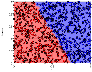
This first sample shows the result of a nearest mapping. Each point of the plane is assigned the class of the nearest sample of the training set. The training distribution is a simple linear split along the y = 1.5 - 2 * x axis.

A zoom in on the boundary between red and blue clearly shows the effect that single samples have on the form of the region.
Patterns analysed
We will now look at the patterns of the independent variables that we will use.
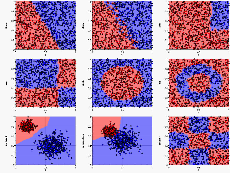
The set consists of eight different patterns:
- linear :
- simple linear split
- nlinear :
- linear split with noise
- and :
- Combining an independent X-Range and Y-Range using an and condition
- xor :
- Combining an independent X-Range and Y-Range using an exclusive or condition
- circle :
- Inside or outside of a circle
- ring :
- A ring formed by an inner and outer circle
- twoblocks :
- Two non-intersecting blocks with normal distribution, that overlap in X and Y range
- mergeblocks :
- Two intersecting blocks with normal distribution
- checker :
- A 3x3 checkerboard pattern
The nearest mapping works fine in most cases, but has a fractured border in most cases. This can be smoothed by using more than one near sample – which is the common K-Nearest algorithm. Using more samples creates a smoother border, but results in more failed classifications of the original set.
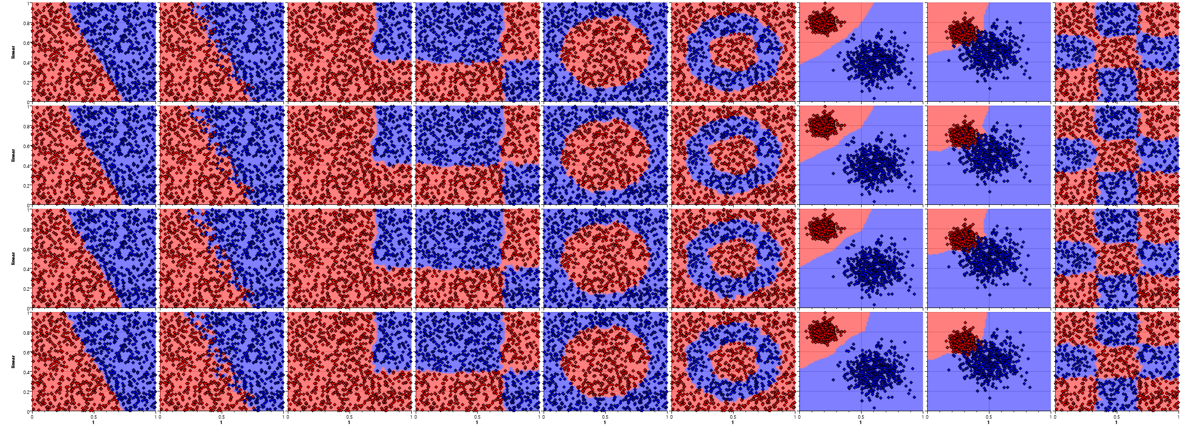
The downside of the K-Nearest approach is twofold. First it requires the complete training set for the prediction and second it is usually quite slow, because it has to find the nearest samples in this training set for each of the samples to predict. We also do not gain any knowledge by using this algorithm. The upsides are no need for a separate training step, ease of adding new training samples later on and the ability to match almost all kinds of distributions.
Classification Algorithms
We will now take a look at the other algorithms.
- dtree :
- Simple decision tree
- bayes :
- Naïve Bayes
- logreg :
- Logistic regression with a linear kernel
- logreg2 :
- Logistic regression with a quadratic kernel
- logreg4 :
- Logistic regression with a fourth order polynomial kernel
- rulelearn :
- Rule learning
- nnet :
- Two level neural network
- svm2 :
- Support vector engine with a quadratic kernel
- svm4 :
- Support vector engine with a fourth order polynomial kernel
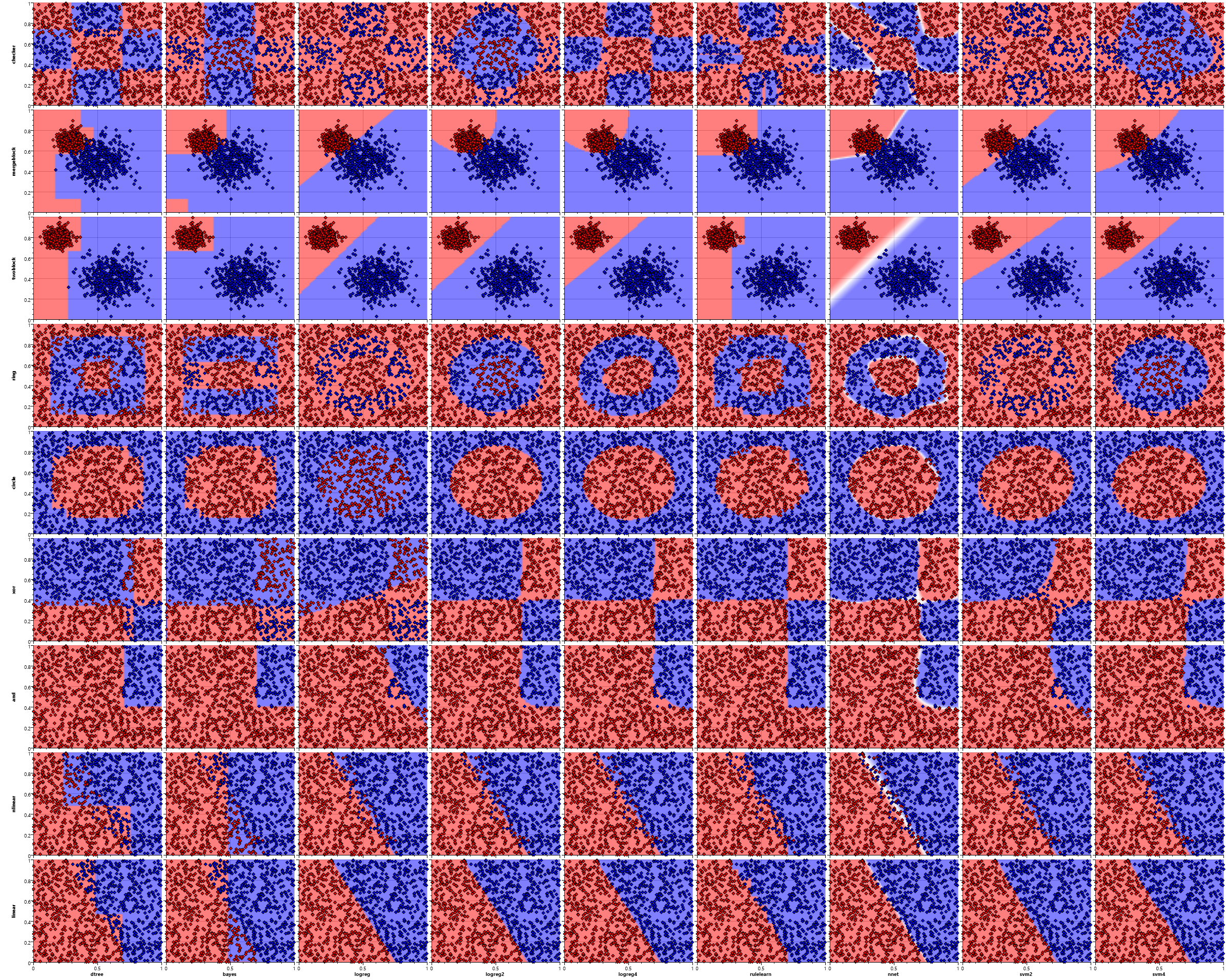
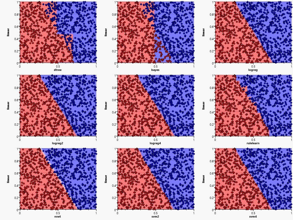
We can already derive some features of the algorithms by looking at the simple linear distribution:
- dtree, bayes and rulelearn have to quantize the feature space
- bayes is not able to detect the dependency between the two variables, thus not able to model the slope
- the neural net has an area of uncertainty (shown as white) where neither the red nor the blue end neuron fires
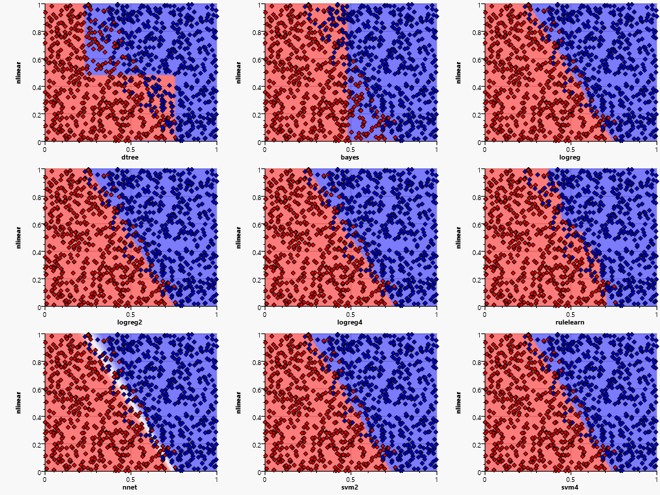
Adding noise to the sample distribution has almost no effect on the logreg and svm based algorithms, but shows an increased area of uncertainty in the neural network. The rulelearn follows an "assumed" border by adding more and most likely superfluous rules, thus requiring some fine tuning of the training parameters.
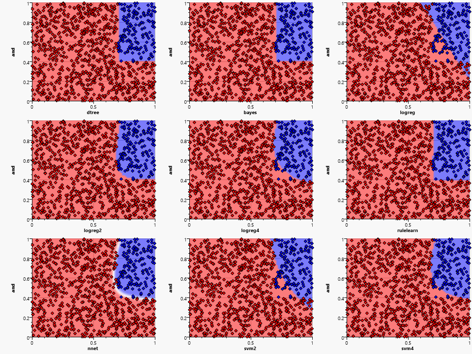
The and pattern works fine with dtree, bayes and rulelearn due to their need for splits on single variables. The logreg fails because it is unable to generate a single separating line – the higher dimension kernels work better but are still unable to generate a perfect fit. The nnet generates a good approximation of the rectangular area.
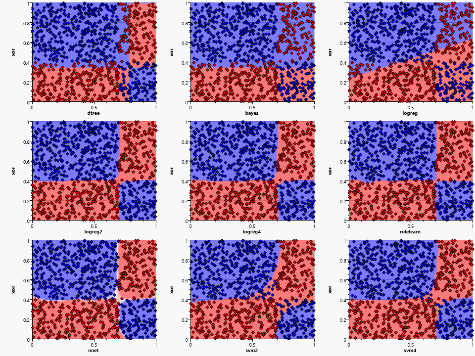
The xor pattern shows the major problems of the bayes and the logreg algorithms and their limited ability to generate complex classification shapes. The bayes algorithm uses a combination of independent probabilities for each dimension and is thus not able to combine the two contradicting probabilities for each dimension caused by the checkerboard pattern.

The dtree, bayes and rulelearn are all able to generate a discretized approximation of the circular area. The simple logreg fails completely. The higher dimension kernel algorithms are all close to the actual circle space. This is expected due to the polynomial structure that is able to model an Euclidian distance function. The neural network generates a somewhat circular form, but has various dents due to the randomness of the training data.
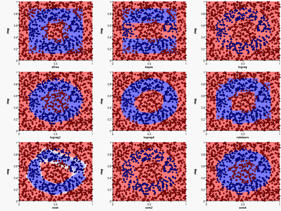
The ring pattern is problematic for most algorithms except for the fourth order polynomial logistic regression, the neural network and the rulelearn. A ring is a natural form for a plane intersecting a fourth order polynomial, the close match is therefore an expected feature of the logreg4.
The nnet could use more training samples (or more training epochs) to form a better approximation, but is still close to the original ring. The actual shape may vary from test to test due to the random starting values of the neurons.
Rule learning and decision tree are somewhat similar, but the rulelearning shows its advantage of being able to have several decision layers and not just one per independent variable.

All algorithms are able to classify correctly for the two separate blocks – although they generate different regions. The bayes shows its preferred and combination, the dtree and rulelearn the need for discretization. The variation in the placement and slope of the separating curve/line for the others shows the need for a training set that covers all edge cases – thus removing the area of uncertainty caused by unpopulated space.
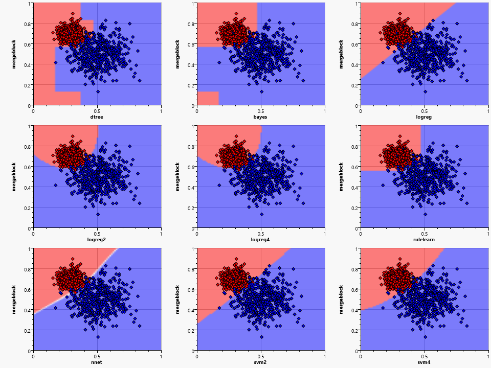
Things get a little more complex when the two clusters overlap, but all algorithms are robust enough to handle this situation. The shape of the classification areas gets more complex and diverse. The same training data can thus result in completely different classifications with different algorithms.
The final example is the checkerboard sample:

The best result is again generated by the higher dimensional logistic regression, the neural net and surprisingly the decision tree. Rule finding suffers from the small sample set, but generates a somewhat covering result.
Conclusion
After looking at all these samples, it appears that the two winners are neural networks and higher dimensional polynomial regression. Unfortunately both come with their own set of drawbacks. Neural networks tend to be slow learners and the outcome depends on the initial random neural factors. Higher dimensional polynomials have an exploding cost regarding the number of independent variables.
Here are some things to take away from this experiment:
- Picking the right classification algorithm requires some experience or a huge number of experiments with different splits into training and validation data sets.
- A lower number of independent variables but a higher order algorithm may lead to a better classification with the same computational effort
- Algorithms that require a discretization step (such as decision trees) might benefit from added knowledge applied using manual discretization
- Neural networks are great classifiers for continuous value spaces but may be overkill for many classification problems
- There is no one size fits all, the same training set may lead to different classification sets with different algorithms
- Make sure that the training set covers most areas of the value space to avoid large regions of uncertainty