Predictive Analytics
Predictive Analytics is used to determine unknown data from known data. For example, this can be methods based on time, extrapolating future or unknown values (dependent variables) from known values of the past (independent variables) or predicting missing data elements by calibrating with complete data set.
In most cases a predictive analysis is not entirely correct since it works with assumptions and non-existing data, but frequently it can improve the data quality or at least increase the subjective amount of information.
The predicted and the existing data attributes can be either continuous (real numbers) or discrete. The case of the value to be predicted being discrete is also called classification – a special case is the binary decision where only two choices are preexisting for prediction (positive – negative). In contrast, methods of regression attempt to approximate the parameters of a mathematical function to a data set such that they yield the best possible mapping of the given independent variables to the dependent variables. These methods are employed for the most part if both the dependent and the independent variables are continuous.
ANKHOR offers various operators for classification and regression:
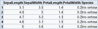
Let us demonstrate four of the most important classification operators by means of an academic example, which is the classical data set of classifying Iris flowers by Sir Ronald Fisher. In this, four continuous features of the flower size are used to discriminate between three subspecies.
_-_Flickr_-_Andrea_Westmoreland.jpg)


The first step for an analysis is always to obtain an overview of the data structure and possible connections. This is facilitated by the "dcanalyzewizard" wizard operator. Its upper part delivers a summary of the data of each column, while the lower part displays the correlation among the columns.
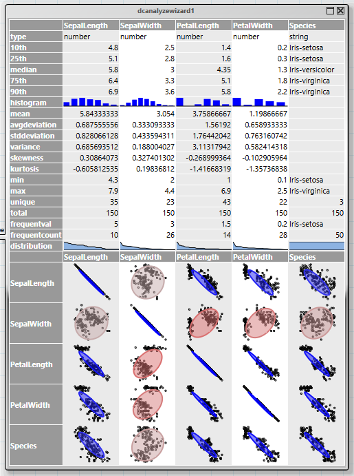
The correlation display combines two forms of diagrams, a scatter plot and an ellipsis. The ellipsis becomes flatter with increasing correlation of two values. Uncorrelated columns appears as circles, complete correlations are closing in as diagonals. It is evident in this example that all flower sizes apart from "SepalWidth" strongly correlate with the species.
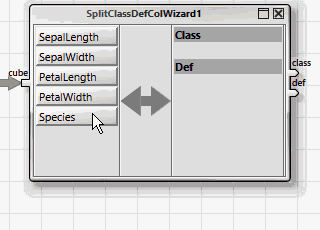
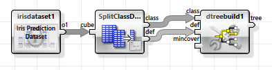
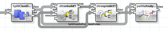
All ANKHOR operators for classification expect the dependent and independent variables in two separate tables, "class" for the dependent and "def" for the independent variables. This can be achieved easily with the help of the wizard operator "SplitClassDefColWizard".
The simplest learning method for classification uses a decision tree, which is created with the "dtreebuild" operator.
The decision tree is evaluated from the left to the right. At the inside nodes one of the branches is taken by means of an independent attribute, finally leading to a decision about the dependent attribute at the leaves.
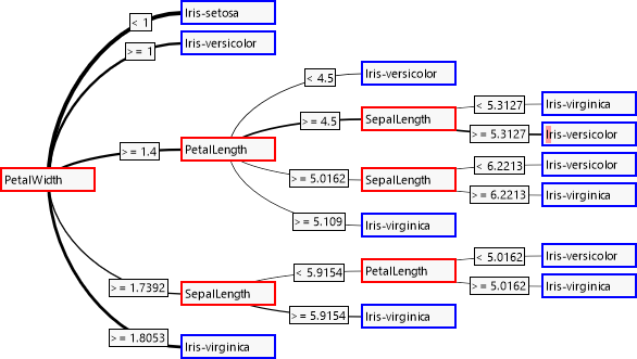
As could be expected with the correlations, the attribute "SepalWidth" is not considered during decision. The connection's thickness reflects the frequency of taking a branch. The small red bar in the fourth leaf indicates that an erroneous classification was carried out for it.
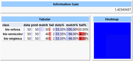
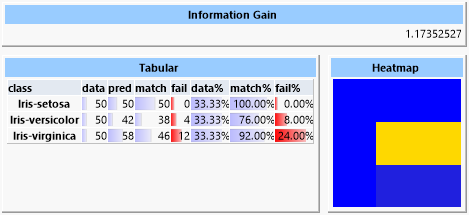
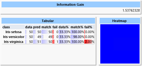
A detailed analysis of the decision tree can be executed via the "paiVisAnalyse" operator. For this we determine all of the dependent values of the data set from the independent values by means of the decision tree and compare them with the actual values.
The result shows various information:
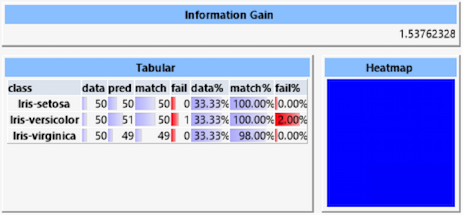
The "Information Gain" is a measurement for the information gained by the prediction. This value grows with the accuracy of the quality of prediction. However, the maximum gain can be limited by low amounts of inherent information caused by a possibly imbalanced distribution of the classes in the data set. The "Heatmap" displays the deviations of the predicted classes to the actual classes. Because in this case the prediction is almost perfect the heat map is uniformly blue. The table lists values for each of the classes:
- data: Number of data sets with this class
- pred: Number of data sets for which this class was predicted
- match: Number of correctly predicted data sets
- fail: Number of data sets erroneously assigned to this class
- data%: Percentage of this class of the data set
- match%: Percentage of correctly predicted data sets
- fail%: Percentage of data sets erroneously assigned to this class
A related algorithm for classification is based on learning logical rules ("rule finding"). These rules have the form of "and" combinations of simple relations. The operator "mrulelearn" delivers a list of rules that can be processed from top to bottom. Each rule is associated with a class and the first rule evaluated as true determines the class assigned.
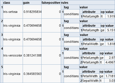
But in contrast to a decision tree the rules can also be considered independently in order to calculate their contribution to the prediction.
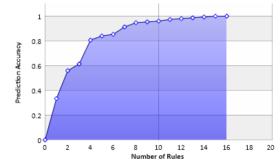
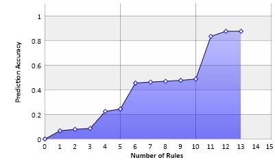
This diagram shows the accuracy of the prediction depending on the number of rules employed. With 16 rules a decision of one hundred percent can be made, but each of the last three rules only covers a single case.
Another very simple classification algorithm is based on conditional probability. The "Naive Bayes" approach assumes that all independent variables are also independent from each other, i.e., they do not affect each other in the probability of class selection.
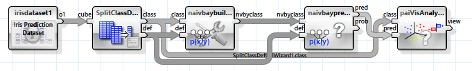
In this example the result of the prediction is only slightly worse than the decision tree's, but the algorithm itself is much simpler and also suited for very large data sets with huge amounts of independent variables.
Linear discriminant analysis and logistic regression are two related algorithms based on linear separability. Here the classes are discriminated by means of hyperplanes established in the N dimensions of the feature space of the independent variables.
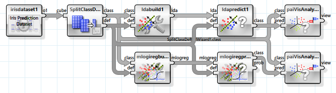
But as the data is not completely linearly separable these methods yield a clearly worse result. Especially the linear discriminant analysis is not suited for this type of problem.
In the heat map the frequent misclassification of the elements of the "versicolor" and "virginica" classes is noticable. The heat map shows correct predictions as blue and wrong predictions as red. Between these boundaries we have green, yellow and orange. The heat map row corresponds to the actual class and the column to the predicted class. So it is obvious that the classes "setosa" and "verginica" could be assigned properly, but the elements of the "versicolor" class were often erroneously classified as "verginica".
A substantially more powerful approach also based on linear separability is the "support vector machine". With the help of a non-linear mapping function the independent variables are transferred into a higher dimensional space, which possesses better prospects of separability. In this example a mapping with a polynomial kernel is used. As the number of dimensions can be huge (even infinite) the mapping is not actually executed but instead a trick is employed with which the result of a scalar product of two feature vectors in the target space can be directly calculated. Thus not the parameters of the separating hyperplanes are stored but support vectors from the set of feature vectors.
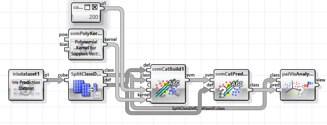
Several parameters can be used to configure the classifier.
A support vector machine is very effective in determining the classes but also requires a long training period, the length of which grows disproportionately with the amount of training data.
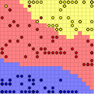
Let us focus on self-organizing maps as the last algorithm mentioned in this document. In the first step these are trained unsupervised (that is, without knowing the dependent variable) to a mapping method from a multidimensional feature space to a two-dimensional chart. In the second step this reduced feature space is then colored according to the class of the data elements dominating that area, so that finally a prediction can be executed by mapping and directly looking up the chart.
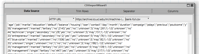
A complicated example with real world data is based on the results of a telemarketing campaign of a bank (source: http://archive.ics.uci.edu/ml/datasets/Bank+Marketing ). The table contains several parameters concerning the customers of the bank and the information whether calling the customer on the phone led to selling a product. The aim of the prediction is to create a classifier with which the group of customers can be restricted such that the probability of a sell is increased and thus the marketing action can be employed more effectively.
The first step is to read the data, which is available as a CSV file in a ZIP archive. This is easily done with the "CSVImportWizard" operator, which executes both downloading the data and converting it into a table.
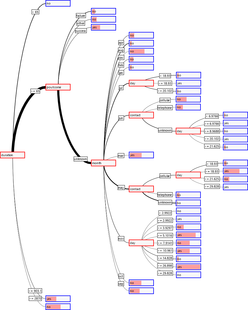
A first look at the correlations between the single independent variables and the dependent variables shows that three of the variables can be categorized with a high probability as particularly relevant for the classification: "duration", "poutcome" and "month".

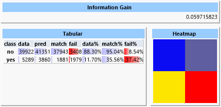
A first attempt with the "Naïve Bayes Predictor" shows an information gain of about 0.06.
In contrast, a decision tree yields an information gain of about 0.22.
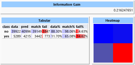
The reason for this is obvious at closer inspection of the tree because it contains almost 6000 leaves, thus it approximated very closely to the data. It is doubtful that this tree would be nearly as successful with different data.

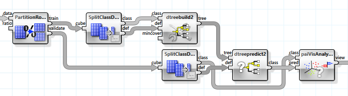
In order to evaluate how good the prediction would be for not exactly the same but similar data, we split up the data set into two parts, one for training and one for evaluation, and use these parts accordingly.
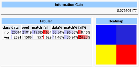
Now the information gain is reduced to only 0.05 with the tree still containing about 4500 leaves. In order to gain a more universal tree we set the "mincover" value, i.e., the share of the data set that each leaf must cover, to 4% (this value was established experimentally). Now the tree possesses only 39 leaves but reaches an information gain of 0.079.
Looking at the tree we observe that the expected variables are close to the root.
For comparison we finally consider a prediction with rule finding.
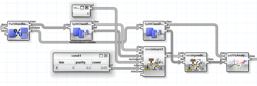
The values for "purity" and "cover" were determined experimentally. The result is an information gain of about 0.11 with 13 rules discovered.
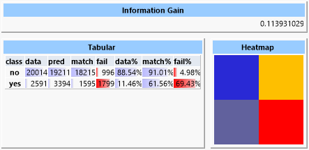
It is obvious that only a couple of rules dominate the prediction.
Even so the information gain in this example is only small, the rate of correct hypothetical classified data is significantly higher for both the "yes" and the "no" cases than a pure random distribution (61.56% against 11.46% in the positive case). Therefor the goal of reducing the group of customers, but with increased probability of success, is achieved.
Of course, the small information gain also originates in the data set having imbalanced density for the two classes due to the low amount of inherent information.
Classifiers in ANKHOR:
| Methode | Types | Advantages/Disadvantages |
|---|---|---|
|
Decision tree |
Arbitrary |
|
|
Rule Finding |
Arbitrary |
|
|
Naive Bayes |
Arbitrary |
|
|
Random Forest |
Arbitrary |
|
|
Closest Neighbour |
Continuous |
|
|
Support Vector Machine |
Continuous |
|
|
Neuronal Net |
Continuous |
|
|
Linear Discriminant |
Continuous |
|
|
Logistic Regression |
Continuous |
|
|
Self-organizing Map |
Continuous |
|