Throwing Darts in Monte Carlo
I recently stumbled over a Blog post "A geek plays darts" talking about the ideal aiming point in Darts for various skill levels of players. Throwing darts is a stochastic process with a two dimensional normal distribution around the target spot (at least in an idealized world without systematic errors).
Determining the expected score for a target spot would mean integrating over the score for each field multiplied with the 2d normal distribution function with the center at the target and a standard deviation based on the player skill. For a full map of all potential targets on a dart board one would need to repeat this for every grid point.
While it is quite simple to calculate the distribution function for any given point and also to determine the score, it is problematic to do so for all points in a closed form. So this will need some form of numeric integration. Integrating with a fixed size grid is problematic (although quite efficient using FFT based convolution), it would have to be small enough to cover enough of the smaller fields and sharp score edges on the board, but then it would spend a lot of computation effort to integrate over parts of the distribution function that contribute only little to the effective integral.
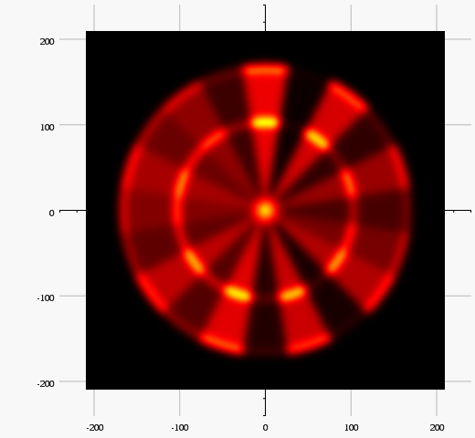
This can be seen with the following chart, which shows absolute errors with different grid sizes (vertical center axis going through the triple 20 at 2mm standard deviation).
A grid with a spacing of 0.16mm has 6.7 million grid points.
A better way is to use Monte Carlo integration by generating samples using the distribution function. This way we will get more samples in the area where the dart is more likely to hit and thus a better result with a lower number of samples.
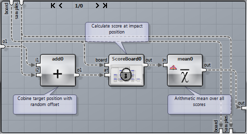
The sheet uses a common set of sample offsets for all integration points to reduce the cost of evaluating the accumulated inverse normal distribution. It is split into six major macros, with most of the work performed in the “Simulate” macro.
The shared offset sample set is generated in the “Samples” macro:
Independent normal distributed samples in X and Y direction are combined into a 2D sample set.
The “Simulate” macro iterates over all grid points in the field, adds the offset samples and calculates the average score:
The grid has to be small enough to cover enough area of the smaller target fields. This is more important for skilled players with a small standard deviation. The numeric quality of the generated integration for players with a larger deviation will benefit more from a bigger set of samples, because they are more likely to hit a larger set of fields, whereas the exact aiming point is not so important.
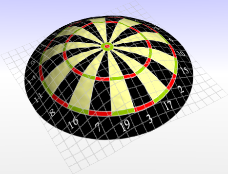
There are various options for displaying the resulting function such as heat maps, contour lines or a 3d surface with the height.
I decided to go with the third option and some additional eye candy ny using a dart board itself as a texture.
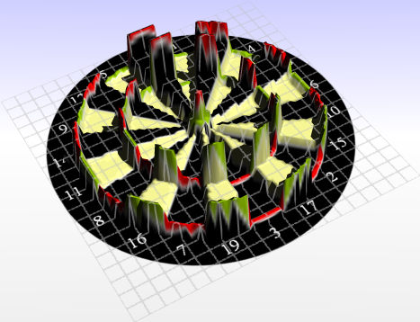
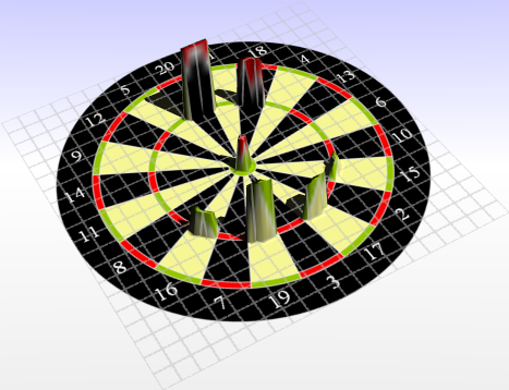
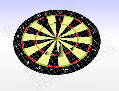
This chart shows the expected scores for an excellent player with a standard deviation of 1mm. The height resembles the actual score of the underlying fields, because the player will almost always hit its target. The next chart shows the score for a poor player with a 10mm standard deviation.
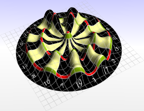
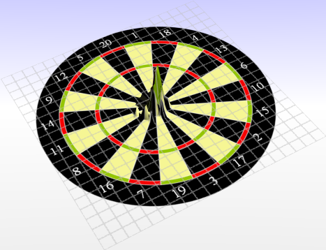
The surface is much smoother because the score of individual fields start to bleed into each other. Even aiming outside the board now promises some points. With a deviation of 50mm the aim should be close to the center, hoping not to miss the board at all.
Starting with a base elevation of zero points is not very helpful because one usually scores some points regardless of aiming (as long as you hit the board). We want to emphasize the ideal target spots, so I am confining the displayed range to the 99th percentile up to the maximum. This way one can see the interesting areas of the board. All other values are clamped at the bottom surface to improve the location cues given by the dartboard texture.
A player with perfect aim should always go for the triple 20.
This is still the case for a 1mm deviation, but the pikes are already smoother.
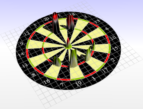
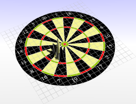
Players with a 5mm standard can still expect to achieve the highest score by aiming at the triple 20. The bulls eye becomes more interesting as a target.
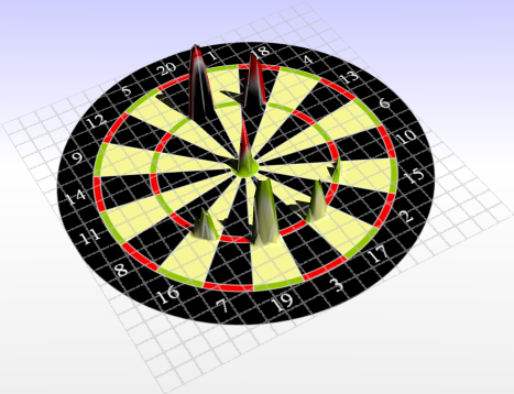
The 18 becomes an irrelevant target at a standard deviation of 10mms. Players should start to look for the triple 19, the risk of hitting the low score fields close to the 20 become higher.
Now at 20mm a player should rather go for the tripple 19. The bulls eye has vanished as a good target spot from to 99% percentile area.

With a 50mm standard deviation the spot moves to the lower left center around the 16.
And with 100mm it is best to go almost straight for the bull’s eye (31.8mm diameter) with a slight shift to the lower right. No more fun with the triples, it becomes simply very unlikely to hit those small fields (8mm diameter). The chart becomes quite rough, with several peaks. This is caused by the 99% percentile scaling, which covers a smaller score area with a higher standard deviation, because scores are distributed more evenly over the board.
An interesting question that remains is, whether the distribution of the impact points is really a normal distribution with the same standard deviation in horizontal and vertical direction. I usually find it much easier to hit close to the horizontal aim but much harder in the vertical direction. This might be due to the way I throw the darts (using the elbow as the major joint) . I would be interested to know whether this is a common perception, and if so it would make sense to repeat the experiment with different values for the two dimensions. Your comments are welcome!
You can also download my FlowSheet implementation below. Please make sure that you use the latest version of ANKHOR FlowSheet for it to work properly. Tip: After loading the file in ANKHOR FlowSheet, right-click over the graph area and select "Show Operator Comments" from the context menu to get additional help on the implementation.
Download FlowSheet (ZIP archive)