Visualizing Compiler File Sizes using Sankey Diagrams
A C/C++ compiler (and other compilers too) generate various intermediate, debug and executable files during a compiler run. Most programmers do not look at those files nowadays unless something is broken, so some years ago I lost the feeling for the sizes of these temporary files (in the old days, when double digit kilobytes was a lot, those sizes did matter quite a bit).
When transitioning to Visual Studio 2013 I had to look at the intermediate files to get some of the conversions correct, and thus noticed the file sizes.
Acquiring the Data
The compiler and linker generate logs during a build that include all source and target files that were part of the build. So after a full rebuild we have logs that include all source, temporary and final files that are used or generated by the build tools.
The first step of our display pipeline is thus to mine those log files and recursively walk all projects that are part of the solution.

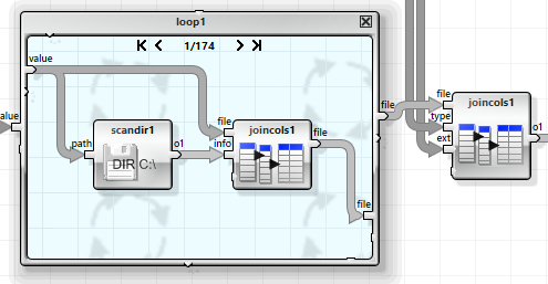
The operator graph is not recursive but uses a while loop that handles one level of recursion per iteration. A list of the log files to consider in the next iteration as well as a list of all files considered so far is passed from iteration to iteration. This way each log file is only considered once, and the loop stops when the deepest recursion layer has been reached.
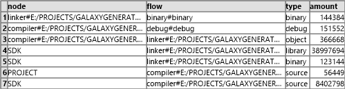
The result is a tag based data structure that has one top level entry per tool run, with sub-entries for the files read, the files written, the name of the tool and the path of the log file.

The next step is then to get the file size and type information for all files that are referenced in this data structure. This is done in three steps. The first step extracts all files from the structure and removes duplicates from the list. he first “forkcols” flattens the top level structure, the second and third flatten it further so only the file names remain.
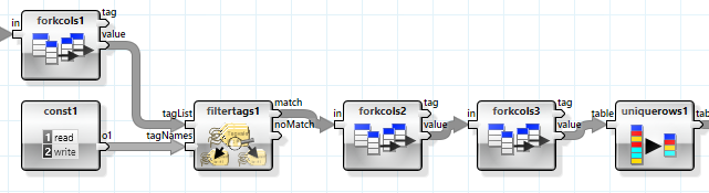
The second step retrieves the file type using the file extension and a lookup table.
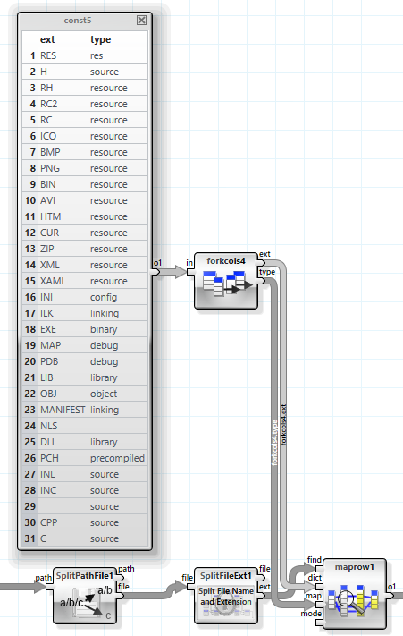
The final step retrieves the file size (and other information, such as the canonical path) for each file in a loop and combines this into a larger table.
Generating Nodes and Flows
A Sankey diagram visualizes flows of arbitrary resources between nodes. Each node may produce or consume any type or amount of resource. In the case of our compiler files the measured quantity is bytes and we will use the following nodes and resource flows:
Nodes:
- Source data sets: SDK for foreign and PROJECT for own files
- Build tools such as compilers and linkers
- Target data sets: binaries, debug, libraries, precompiled headers
Flows:
- Source files, Resource Files
- Object Files, Libraries, Compiled Resources
- Binaries, Debug Data
The general idea behind the node and flow generation is based on production and consumption of resources by nodes. Each log file results in one node and is identified by the path and the tool used.
Two large tables are generated in the following operators that have one row for each such log file and data file consumed or produced.
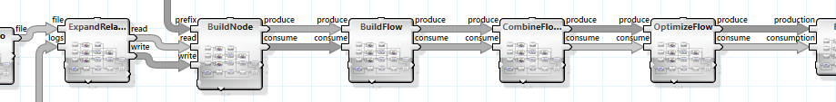
A chain of operators performs various operations on these two tables:
- Create mangled names for all nodes and flows using log file paths, tools and file types
- Sum the sizes of the files of each flow type
- Optimize flows for single producer / consumer cases
The resulting two tables are then simple node / flow relations including the type of flow, the mangled names and the amount of data consumed or produced.
Building the Diagram
The Sankey diagram operator requires node and flow information besides the consumption and production table. This information can be generated from the two tables by combining the nodes from both and taking the flows from the production table (there are no resources consumed that have not been produced).
Format information is added based on the type of resource.
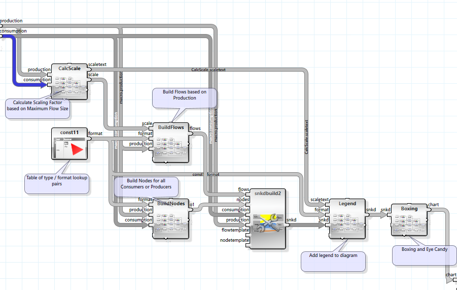
The scaling factor of the resources is based on the maximum flow and scaled to approximately 100 pixels.
A Simple Solution
So let’s first look at a simple solution that consists of one project with a small number of source file.
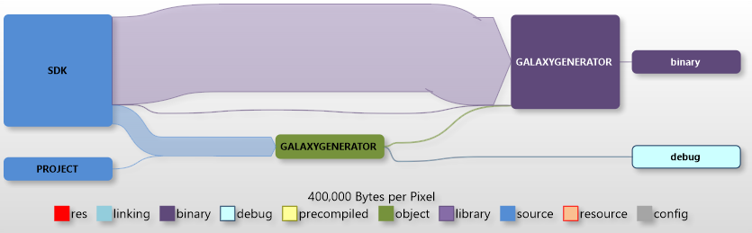
The biggest chunks are the headers and runtime libraries taken from the SDK, but only a small amount of this is kept by the linker. The amount of source seems to be in a good relation to the amount of intermediate and final data. The small green box is the compiler run – the larger purple box the linker.
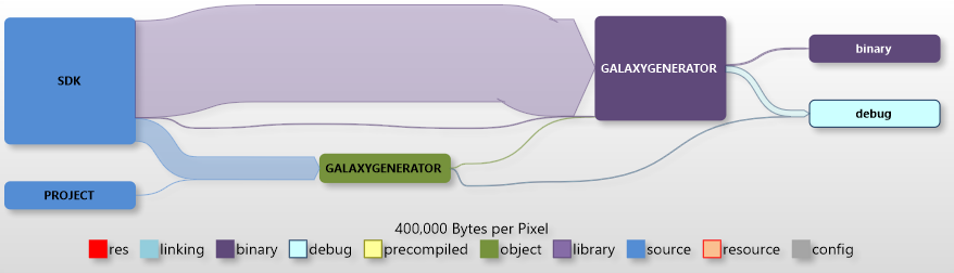
The debug version is quite similar; the only notable difference is the significant amount of debug information generated by the linker.
Headless Server Component
The next project is one of the headless ANKHOR server components, the remote execution server. There is no user interface code and the largest chunk of source that ends up in the project is the ANKHOR in memory execution engine “Tablesolver”.
First we look at the debug version:
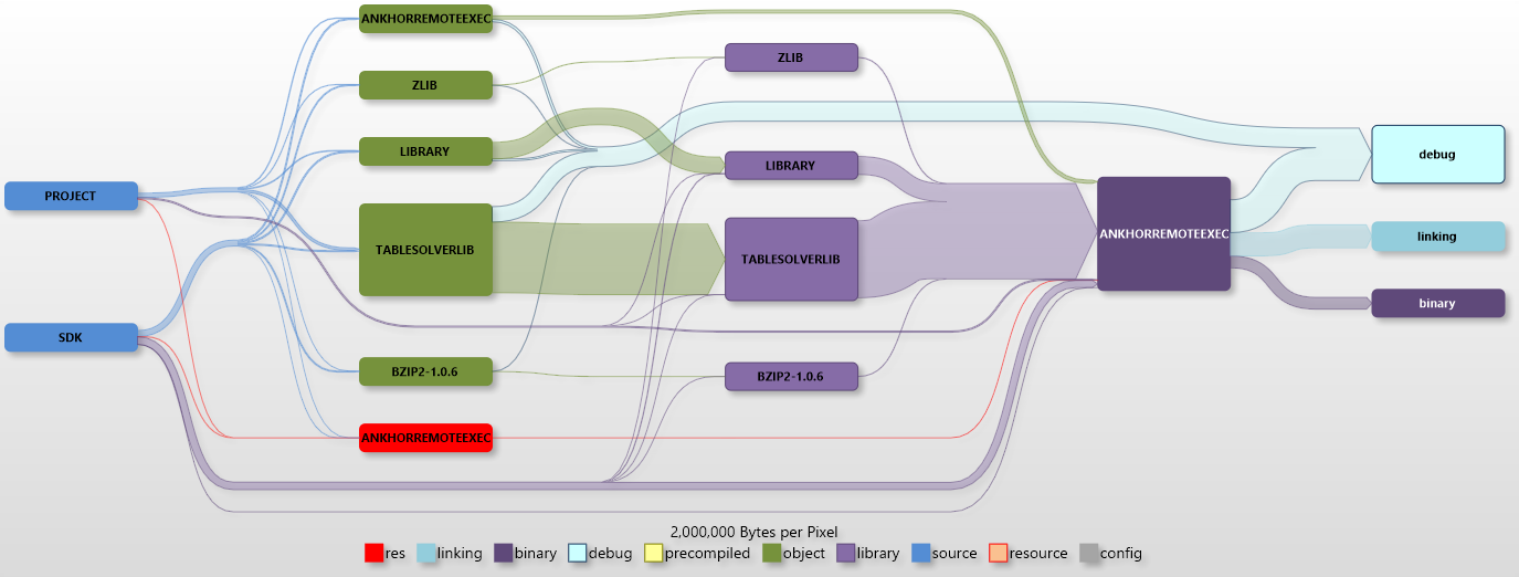
The amount of project generated object files is now significantly larger than the SDK based libraries (note the different scaling). An additional step that was not part of the previous diagram is the static library linker. We can see that there is almost no size difference between object files and static link libraries, but one has to keep in mind that the object files don’t go away when the library is generated, thus we duplicate the size of intermediate data by this step.
The small resource path is needed for the version info.
The size of the generated binary is much smaller than the intermediate size and shadowed by the debug information and the incremental linker file.
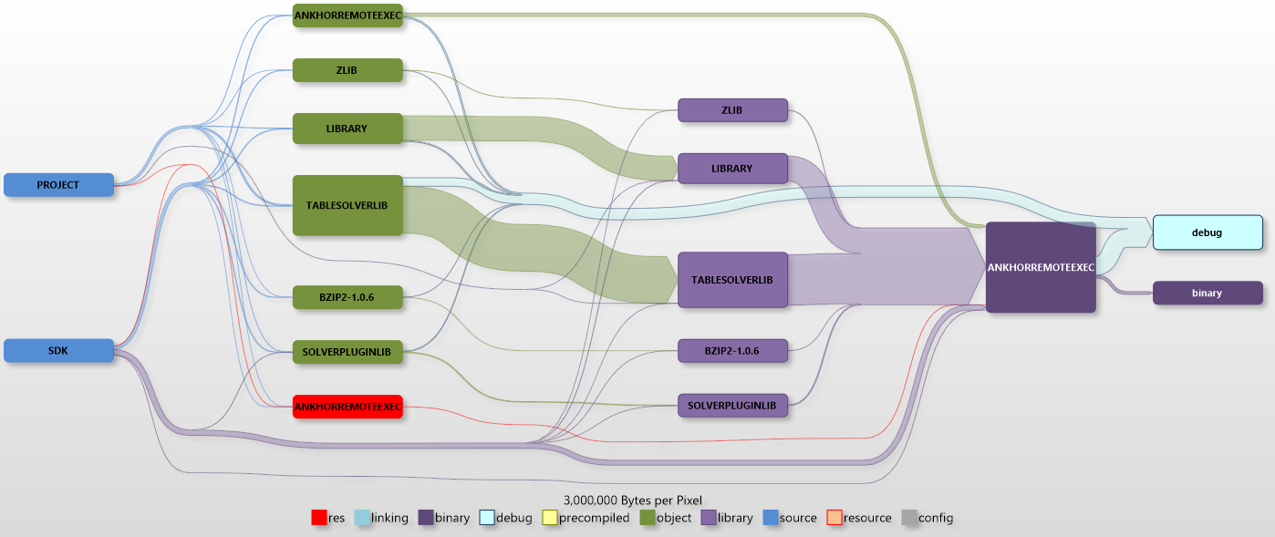
There is no incremental linker file in the release build, but quite a bit of debug information. We keep this information to be able do debug problems in the release builds using dump files.
ANKHOR FlowSheet Application
The next diagram shows the debug build for the ANKHOR FlowSheet application.
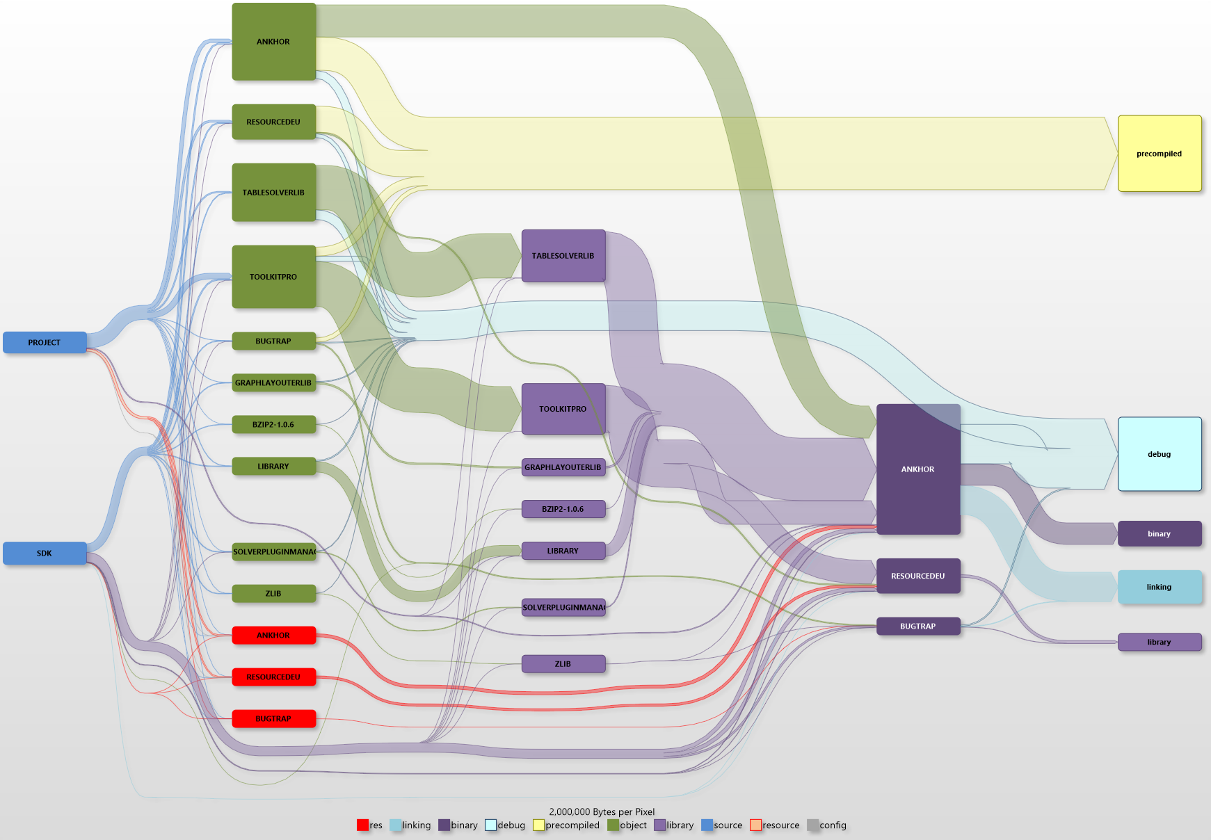
The added complexity is caused by the additional projects - the ANKHOR application code and the GUI toolkit used. here are also three binaries generated instead of only one, the ANKHOR application itself and two DLLs. he compiled resources are now also a more significant part of the complete build.
The yellow flow is composed of the precompiled headers. One can easily see that this block is significantly larger than all sources combined, and only matched by the combined debug data.
Conclusion
The Sankey diagrams do not only show why your hard drive is cluttered with intermediate files, they also helped me spot some fragilities in the build process. Sometimes the build order was not 100% correct and some of the intermediate files ended up in the wrong folders (due to the fact that the projects have been moved through five generations of Visual Studio by now).